Inefficient LLM Serving Problem

The case to move away from "monolithic" to "disaggregated" model serving.

The Efficiency Divergence: Model Training vs. Serving

---

Note: references to “inference” and “serving” are used interchangeably in this article.

Most of the real-world compute in AI today happens after a model is trained, but the economics of serving have not caught up to this shift. A 2025 study of large-batch inference on modern GPUs found something startling:

“Even under batch sizes of 16 or more, GPU compute capabilities remained underutilised — DRAM bandwidth saturation emerged as the primary bottleneck.”

In practical terms: in many real-world inference workloads, GPUs run at less than 40% of their compute peak.

If your cloud bill is mostly GPU-based for inference, this study means you are overpaying for compute that mostly sits idle that the workload is fundamentally unable to exploit.

Don’t be surprised though. This isn’t a glitch. It’s the core flaw in how modern large-batch LLM serving/inference is designed and deployed.

---

Why we are here and why it matters now?

Over the last few years, training large models got more efficient due to advances in model parallelism / tensor-parallel training, mixed-precision math, sparsity, and better hardware have driven down per-parameter training cost per FLOP.

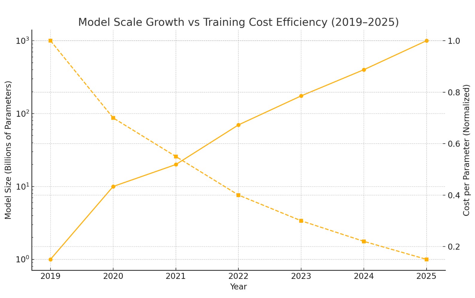
Take a look at the chart below showing model parameter growth vs. training cost efficiency for the period 2019 - 2025.

• Parameter counts are shown on a log scale because growth has been exponential

• Cost per parameter steadily declines representing gains from multi-precision training, ZeRO partitioning, 3D parallelism, etc.

• Optimizers like DeepSpeed with ZeRO dramatically reduces per-GPU memory overhead by sharding optimizer state, gradients, even parameters.

• 3D parallelism that combines data, tensor/model, and pipeline parallelism enables very large models to be distributed across many GPUs, circumventing single-device memory limits while preserving training efficiency.

• Activation / memory optimizations (activation partitioning, memory offload, activation checkpointing) further reduce per-device VRAM usage, enabling larger models without prohibitive hardware demands.

In many cases, the marginal cost of training additional parameters has fallen, while model quality (per parameter) has improved. That’s why we see rapid iteration cycles, frequent fine-tuning, and an explosion of models.

But there’s a catch:

Once trained, these models need to be served, and serving hasn’t enjoyed the same gains.

• Context windows are ballooning (16K, 64K, even 128K+ tokens)

• Users expect low-latency, multi-turn, chat-like interactivity

• Personalization (adapters, LoRA, retrieval-augmented generation) demands more memory, more state, more concurrency

For many production workloads (agents, chatbots, workflows), inference cost already exceeds training cost over the lifetime of the model.

The root mistake here is treating inference as a single workload.

It sounds simple. But it’s wrong. Because LLM inference is not one workload. It is two — with radically different hardware needs.

• Phase 1: Prefill (understand)

• Phase 2: Decode (create)

We need to understand why these two phases of LLM inference have unique hardware requirements to better appreciate the architecture that solves the inefficient LLM serving problem.

---

The Anatomy of LLM Inference

Let’s understand what happens when you type a question like “Write a poem” into Gemini or any AI chatbot. To us, it feels like a single action: one request → one response.

Under the hood, though, your message triggers a multi-stage pipeline that is much more than a single mathematical operation.

Let’s walk through what actually happens, because understanding this pipeline is the key to understanding why inference costs and performance behave the way they do.

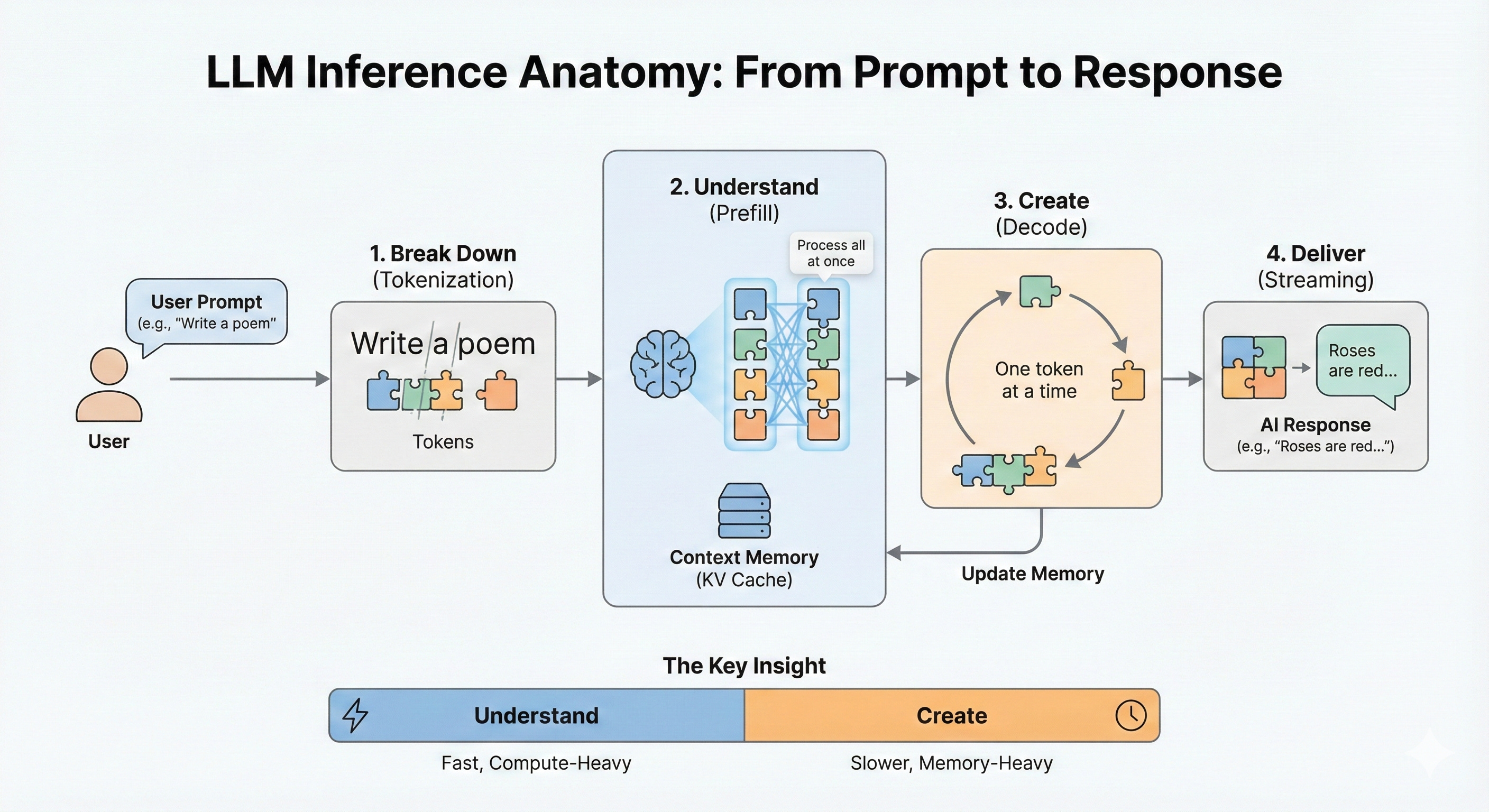
1️⃣ Tokenization

Breaking down language into math

Your text is broken into tokens since the LLM powering the chatbot doesn’t see language, it sees high-dimensional vectors.

Tokens are like jigsaw puzzle pieces for language.
Each piece isn’t the full picture — but the model knows how pieces fit together. Because it has seen millions of examples of similar pieces forming coherent language during training.

Why break language into tokens?

• LLMs have a vocabulary of ~50,000–100,000 such jigsaw pieces

• It knows how each piece connects to others in context

• Any human sentence can be rebuilt from these bricks

This is why pricing and limits are per token as they reflect the actual amount of language the model processes.

2️⃣ Prefill

Processing and understanding the entire input prompt

The model ingests the full set of input tokens all at once (or say, parallelized).

Every transformer layer performs:

• Multi-head attention

• Feedforward projections

• Dense matrix multiplications across every input token

This is where the model builds understanding:
What are you asking? What do you want? What’s relevant?

Outputs of this stage are stored as internal state called Key-Value (KV) cache - the model’s working memory for your request.

What is KV Cache? The “keys” and “values” represent contextual embeddings for each token, needed to compute attention for future tokens. More tokens → exponentially more memory → KV cache often dominates VRAM budgets.

3️⃣ Decode

Generating the response, one token at a time

The model begins autoregression:

Predict next token → append to prompt → repeat → repeat → repeat…

For each output token:

• The model accesses the entire KV cache so far

• Performs small attention + FF operations

• Writes back updated KV state

This continues until:

• A stop token appears, or

• Output reaches max generation length, or

• You interrupt (e.g., user stop)

Decode is sequential — each token depends on the last.
Unlike prefill, we can’t parallelize it.

4️⃣ Streaming

You see words as they emerge

Modern UX streams tokens as soon as they are generated:

• Fast feedback → better engagement

• But requires that the model compute in real time

This magnifies the importance of:

• Memory bandwidth

• Latency consistency

• Efficient state movement

5️⃣ Multi-Turn Statefulness:

Handling conversations, not just queries

You ask follow-ups:

“Can you make that more technical?”
“Summarize in 3 bullets.”

These rely on previous output + original context.

The KV cache grows as you continue the conversation — keeping memory as the primary bottleneck.

---

The Big Insight

LLM inference is not:

“Run the model once.”

It is:

A two-stage, state-carrying process where the dominant bottleneck changes mid-flight.

• Prefill → compute-bound (because the model processes entire input prompt in one pass)

• Decode → memory-bandwidth-bound (because the model generates output tokens, one at a time, using Key-Value cache)

Understanding this duality (along with the hidden KV cache tax) is the key to fixing inference economics — because different silicon is optimal for each stage.

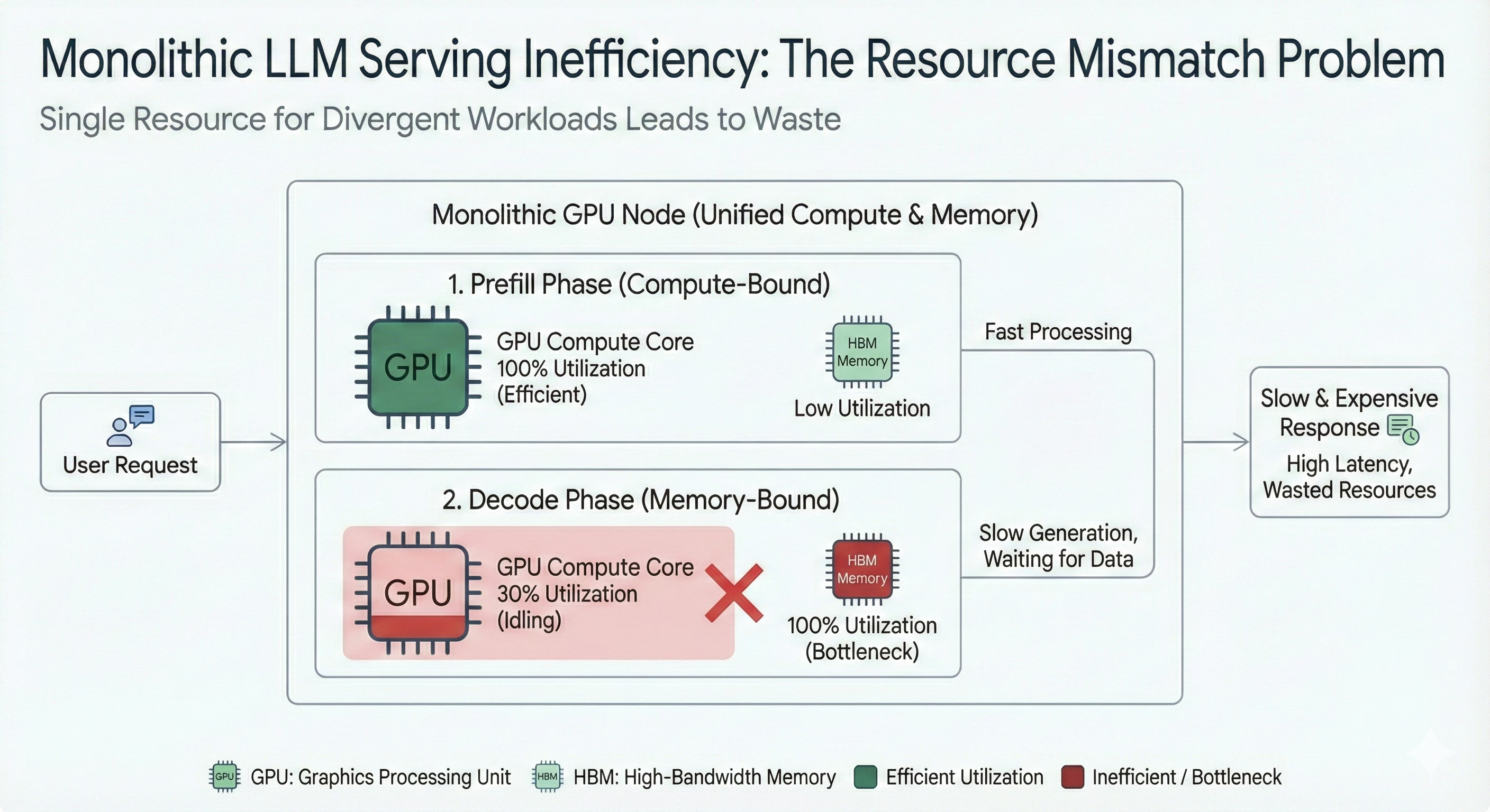
• Prefill underutilizes memory bandwidth (wasting HBM potential)

• Decode underutilizes compute (tensor cores stall)

When you smash both phases onto one GPU, you pay for peak compute while the actual job is waiting on data. That dissonance is what makes monolithic model servers disastrously inefficient at scale.

Academic and industry analyses confirm this inefficiency:

• A recent in-depth GPU-level analysis of large-batch inference by IBM shows that even with large batches, memory bandwidth — not compute throughput — is the bottleneck, leading to underutilization of core compute units.

• Some reporting indicates that many AI-accelerators see < 50% utilization during inference — meaning a large portion of the hardware potential remains idle while the user waits.

• According to this Nvidia Developer Forum discussion, for transformer-based LLMs under low-batch or long-context decode workloads, the theoretical “arithmetic intensity” (FLOPs per byte transferred) drops sharply — pushing the workload squarely into the memory-bandwidth-bound regime.

Put simply: we are renting more compute-bound hardware than we truly need for LLM serving— because the workload can’t use it.

---

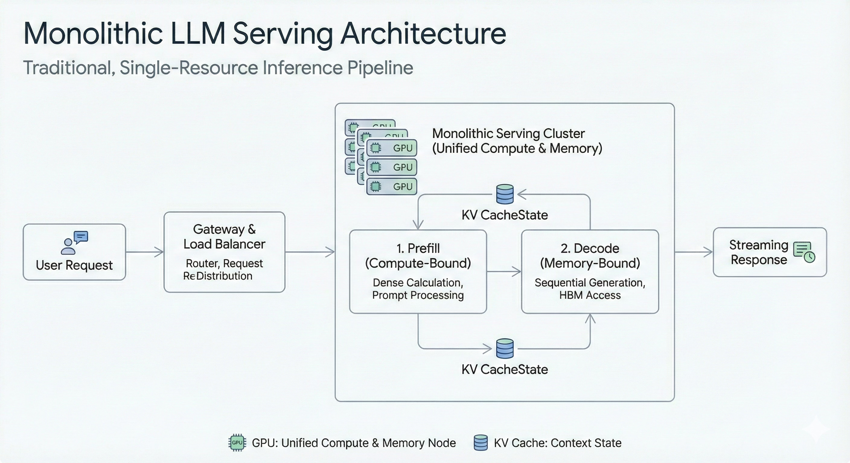
Why Monolithic Model Serving Is the Wrong Trade

When you deploy an entire LLM serving stack as a single monolith (weights, KV cache, decoding, everything), you end up with:

• Compute-heavy hardware idling most of the time

• Huge memory demands (context length, KV caching)

• Inefficient scaling - you scale the whole stack even if only one part is congested

• Worst of all: you pay for peak possible load while actual usage is far below

That model made sense in the early days (512 token contexts, small batch sizes, and stateless requests). But today demands have changed:

• Context windows of 16K, 64K, even 128K+

• Peek-throughput for interactive chat and long generations

• Multi-turn sessions, cache reuse, adapter loading

• Tight latency & cost constraints

The architecture can’t handle that load (not without burning money)!

Take a look at the Roofline chart for monolithic serving: decode lands in the worst possible location for GPUs: low FLOPs/byte → cores stall waiting on HBM. No amount of GPU overclocking fixes decode, because compute is not the problem. Memory is.

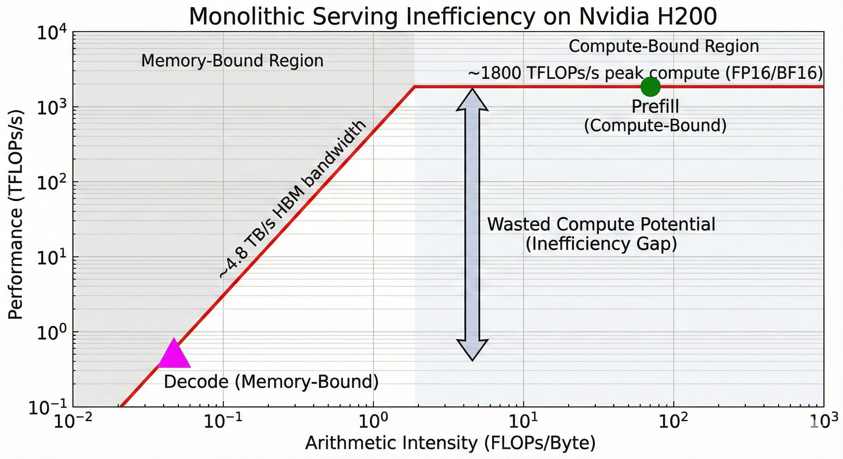
The above Roofline model illustrates the efficiency divergence. ‘Prefill’ (green) utilizes the chip’s peak compute capability, while ‘Decode’ (magenta) is strangled by memory bandwidth, leaving massive compute potential unused.

---

The Solution: Break the Monolith

If the core problem is forcing two incompatible workloads onto the same hardware, the solution is obvious: stop doing it.

We need to move away from monolithic model serving and towards a disaggregated architecture.

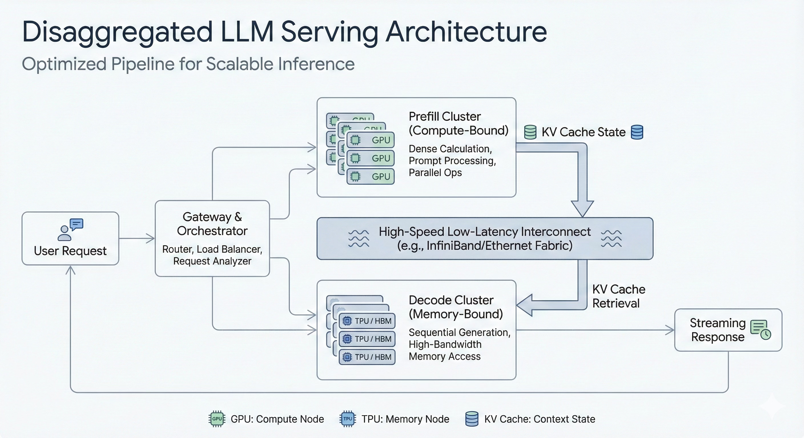
This means physically separating the prefill and decode phases onto different hardware pools that are specialized for their unique requirements.

• Prefill Pool: A cluster of compute-dense GPUs designed to crunch through massive prompts in parallel. Their only job is to generate the initial KV cache as fast as possible.

• Decode Pool: A separate cluster of hardware, like TPUs, optimized for massive memory bandwidth (like High Bandwidth Memory, or HBM). Their only job is to serve the autoregressive token generation loop, keeping the KV cache hot and accessible.

• High-Speed Interconnect: A blisteringly fast network fabric designed to move the large KV cache state from the prefill pool to the decode pool with minimal latency.

By disaggregating the workload, you can independently scale the resources for each phase.

• Have a spike in long-context prompts? Scale up the compute-heavy prefill pool.

• Have a spike in long-form generation users? Scale up the memory-rich decode pool.

You no longer have to over-provision expensive hardware just to meet the peak demand of one phase while it sits idle during the other.

This architectural shift is the key to aligning infrastructure costs with actual usage, finally breaking the cycle of paying for a Ferrari that never leaves first gear.

Why this works

• Prefill stays compute-bound: GPUs crunch through dense math efficiently

• Decode moves into bandwidth-friendly hardware: TPUs or HBM-optimized chips thrive on KV streaming

• KV cache becomes persistent state: reuse across turns, avoid recompute

• Phase-aware routing ensures each request hits the right hardware, even mid-session

Let’s see how this looks on a Roofline chart using an H200 for prefill and a TPU v7 for decode:

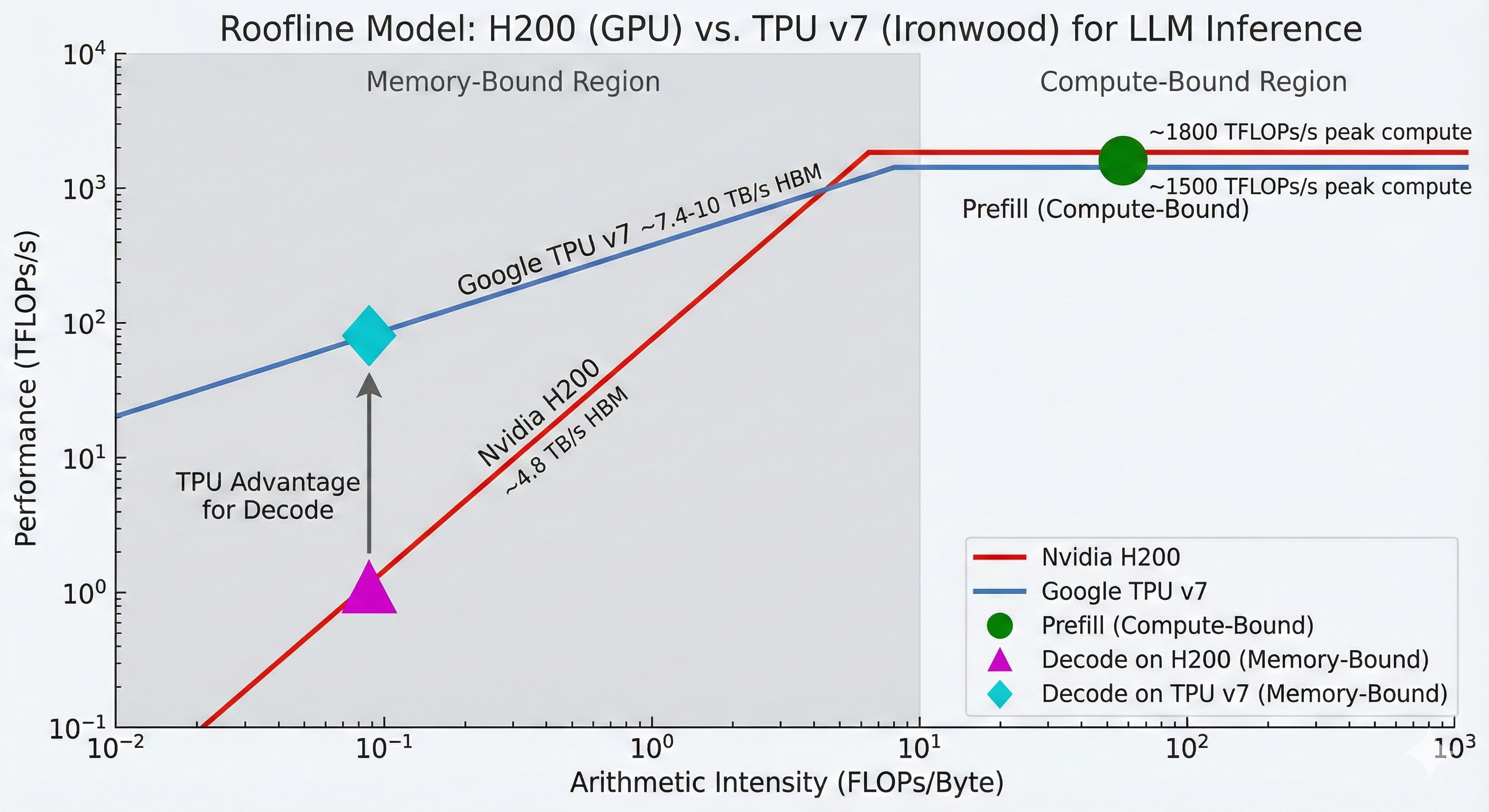
• Both accelerators are compute-bound during the “Prefill” phase,

• “Decode” phase is significantly memory-bound on the H200, leading to suboptimal performance.

• In contrast, the TPU v7, with its higher memory bandwidth, offers a substantial performance advantage for the decode phase, placing it further up the “roofline” in the memory-bound region.

---

The Disaggregated Advantage: A Real-World Example

Theory is nice, but let’s look at the brutal math of a real production workload. Let’s make this concrete with a realistic, high-value workload. Imagine an AI agent that reads a large document and generates a detailed summary.

• Model: 100 Billion Parameters (Dense)

• Input Context: 16,000 tokens (e.g., a 40-page report)

• Output Generation: 2,000 tokens (a comprehensive summary)

• Hardware: GPU (Nvidia H200) + TPU (Google v7 Ironwood)

• Assumptions:

  • GPU hourly rate: $2.50/hr → $0.000694 / sec

  • TPU hourly rate: $1.75/hr → $0.000486 / sec

• Note: illustrative examples to compare monolithic vs. disaggregated serving, not precise or vendor-committed performance or cost guarantees.

Now, let’s compare how this workload plays out on a monolithic setup versus a disaggregated architecture, using today’s top-tier hardware.

1️⃣ Monolithic Model Serving:

Everything — tokenization, prefill, KV cache, decode — happens on one GPU.

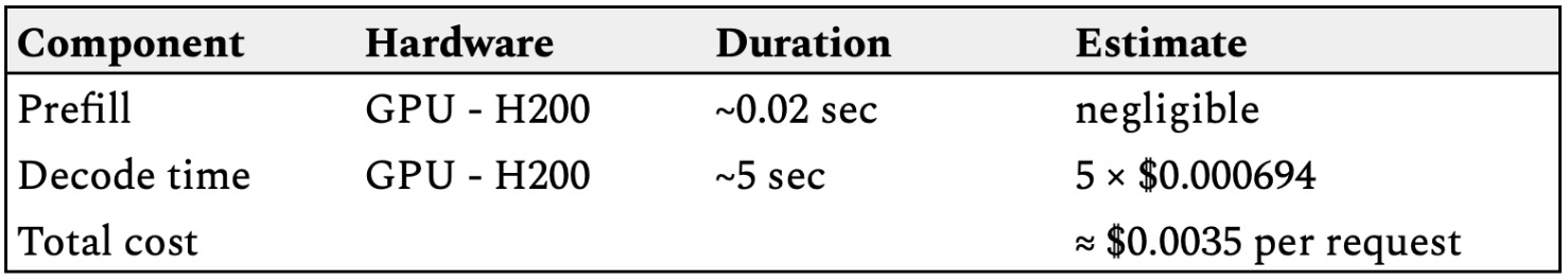
• Prefill: Full 16K context processed in parallel; GPU tensor cores at ~90% utilization; Compute-bound workload → GPUs shine

  • ≈ 100B params × 16,000 tokens × ~2 FLOPs/param

  • ≈ 3.2 × 10^15 FLOPs

  • ≈ 3.2 PFLOPs

  An H200 GPU provides ~1.4–1.8 PFLOPs peak. This is a perfect GPU workload. It saturates the math cores efficiently.

• KV Cache: 70–80 GB per concurrent user session.

  • ≈ (2 tensors) × (96 layers) × (hidden dims ~12k) × (16k tokens) × (2 bytes for FP16/BF16)

  • ≈ 70–80 GB of VRAM

  • ⚠️ Crucial note: This is why “long context support” is so hideously expensive. You run out of memory long before you run out of compute.

• Decode: 2,000 tokens, generated one at a time; each step must read all prior KV cache (≈ 70–80GB); Tensor cores stall waiting for memory

  • ≈ ~75 GB reads/token × 2,000 tokens

  • ≈ 150 Terabytes of total HBM traffic (!!!)

  This is a bandwidth war. The compute cores spend most of their time waiting for memory. On a H200 GPU:

  • HBM BW ≈ 4.8 TB/s → saturates quickly

• Result: Tensor cores stall — ALU utilization drops to ~15–40%

• Cost per request: ~$0.0035

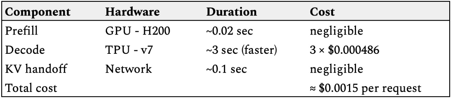
2️⃣ Disaggregated Model Serving:

Split the pipeline into the two natural phases: Prefill → GPU (H200), Decode → TPU v7 Ironwood

• Prefill Phase: on Nvidia GPU (Compute Pool) remains unchanged:

  • ~3.2 PFLOPs in just a few milliseconds

  • Tensor cores running at high utilization (~90%+)

  • KV cache (~75GB) generated exactly once

⚠️Here is where the disaggregation happens in this serving architecture.

• State Handoff:

  • Instead of switching to decode, the GPU’s job is done.

  • The system takes the generated KV cache (~75GB) and transfers it over a high-speed, low-latency interconnect to the Decode Phase.

• Decode Phase: on TPU v7 “Ironwood” (Memory Pool) -

  • The decode pool is stocked with hardware designed to handle the massive HBM traffic.

  • TPU v7, with its massive HBM bandwidth (>7.4 TB/s) receives the KV cache and begins the 2,000-token generation loop.

  • Because its memory pipe is so much wider, it can feed its compute cores much faster.

• Result: >2x reduction in the cost per request.

• Cost per request: ~$0.0015 (2.3x cheaper than monolithic serving)

And the bigger the context?
The longer the output?
The more turns in the conversation?

→ The savings gap widens exponentially.

Because disaggregation aligns physics with economics:

• GPUs do dense compute

• TPUs do memory streaming

• KV cache becomes reusable state, not recompute waste

3️⃣ Cost & Efficiency Impact

Let’s look at the estimated impact on cost per million output tokens for the decode phase, which dominates the total runtime.

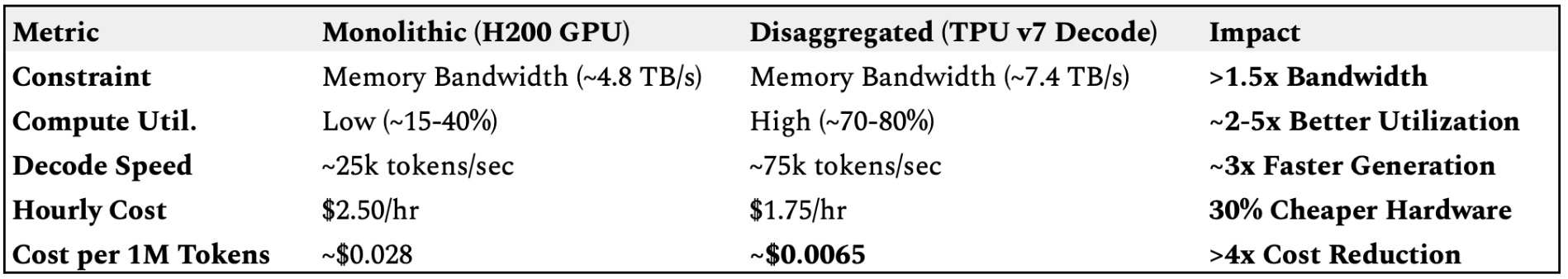
By routing each phase to the hardware best suited for its physics, the disaggregated architecture achieves a >4x reduction in the cost of generation.

Because decode dominates output token generation (especially for long responses and chains), token economics define inference cost.

With disaggregated serving:

• Prefill runs on expensive compute (GPU) → but only briefly

• Decode runs on bandwidth-optimized, lower-cost TPU (or equivalent)

• KV reuse reduces repeat compute & memory pressure

Net effect: 50–80% reduction in $/token for real workloads, especially with long context and high concurrency.

4️⃣ Beyond Cost

While cost is the headline, the other two “silent Killers” of Monolithic Serving making disaggregation mandatory for enterprise production are:

1. “Context Window” Trap:

We are entering the era of 1M+ token context windows. In a Transformer, the KV cache grows linearly with context length. For a 1M token document, the KV cache size becomes astronomical, easily exceeding the HBM capacity of a single device.

• Monolithic: You hit the “Memory Wall” instantly. You can’t fit the batch and the context on one chip.

• Disaggregated: You simply scale the Decode pool. You can stripe the KV cache across multiple TPUs without wasting GPU compute cores. Disaggregation is a leading pattern to serve 1M+ context windows economically.

2. “Stutter” Problem:

In a monolithic server, a new request (Prefill) and an ongoing chat (Decode) fight for the same compute resources. If a user sends a 500-page document for summarization (Prefill), the GPU locks up to crunch that math. Meanwhile, the user in the chat window next door sees their stream freeze. This is called Head-of-Line Blocking.

• Fix: Disaggregation physically isolates these workloads. The “heavy lifting” prefill jobs never block the “fast twitch” decode jobs.

• You get smooth, consistent Time Per Output Token (TPOT) regardless of how many heavy documents are entering the system.

---

How Google Cloud makes Disaggregated Serving real?

On paper, disaggregated serving is obvious. In practice, it is terrifyingly difficult to implement.

If you tried to build this yourself on standard cloud infrastructure, you would likely fail. Why? Because moving gigabytes of hot state between machines mid-request introduces a new, deadly bottleneck: network latency.

If transferring the 75GB KV cache takes longer than the time you saved by using a TPU for decode, you have achieved nothing but added complexity.

Google Cloud is able to productize this architecture not because of a single feature, but because of a decade of investment in three specific areas that solve the physics, software, and orchestration challenges of disaggregation.

1. Physics: Jupiter Data Center Fabric

The primary constraint on disaggregation is the speed of light in fiber.

To make state transfer nearly instantaneous, you need more than just standard 100Gbps Ethernet.

Google’s implementation relies on its Jupiter data center network fabric.

• This is the same infrastructure that allows them to connect 9,000+ TPUs into a single supercomputer.

• It provides massive bi-directional bandwidth and, crucially, ultra-low tail latency.

When a prefill finishes on a GPU, the KV cache isn’t just slowly siphoned over HTTP. It is blasted across a fabric designed for HPC-level direct memory access. This ensures the “handoff penalty” is negligible compared to the decode performance gains.

KV cache handoff is the magic moment.

• GPU pod serializes KV state

• Transfers over high-bandwidth data center fabric (Jupiter networking)

• TPU pod loads directly into HBM

• Decode resumes mid-flight

⚡ Round-trip on Jupiter: Latency-to-first-byte < tens of ms for tens of GB of payload at scale

Attempt that in a commodity VM environment, and you’ll watch the latency bar chart go red.

This architecture requires hyperscaler-grade networking.

2. Software: Unified vLLM Runtime

Historically, running a heterogeneous cluster was a nightmare. You’d need one serving stack for NVIDIA GPUs (using TensorRT-LLM or Triton) and a completely different stack for TPUs (using TensorFlow Serving or JAX native). Moving state between them was non-trivial.

Google solved this by embracing the open-source ecosystem. They built a high-performance tpu-inference backend for vLLM.

• This means vLLM is now the unified runtime layer. It abstracts away the hardware differences.

• It utilizes PagedAttention to manage memory efficiently on both GPUs and TPUs.

• You deploy the same model container, speak the same API, and emit the same metrics, regardless of the underlying silicon.

• The software doesn’t care where the KV cache came from, only that it arrived.

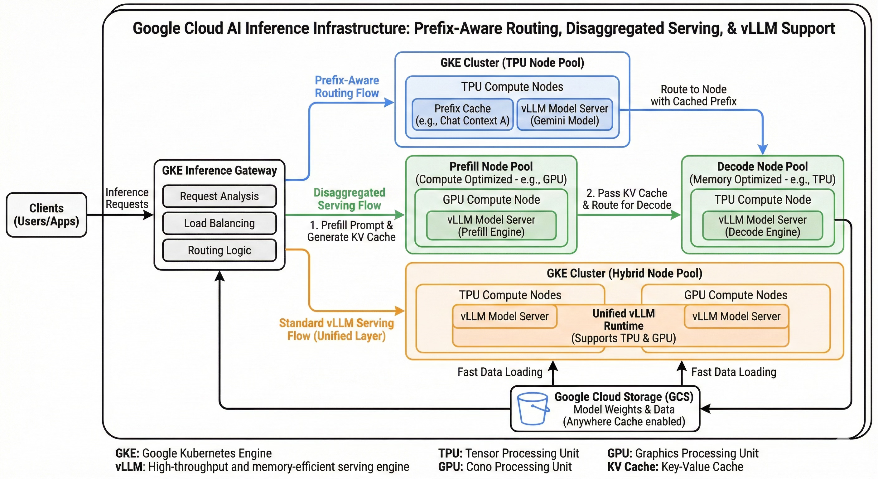
3. Orchestration Solution: GKE Inference Gateway

You cannot manage this complexity with standard Kubernetes Services. You need a control plane that understands the physics of LLM workloads.

This is the role of GKE Enterprise and the new Inference Gateway.

• Specialized Node Pools: You define distinct GKE node pools:

  • One stocked with H200s labeled role: prefill

  • Another with TPU v7s labeled role: decode.

• Phase-Aware Routing: The Inference Gateway acts as the intelligent traffic controller.

  • It knows not just how to route based on URL path, but based on the phase (prefill/decode) of the request.

  • It directs initial prompts to the prefill pool and subsequent decode steps to the memory pool.

• Independent Autoscaling: GKE can autoscale the prefill pool based on compute saturation (e.g., “keep GPU utilization below 90%”) while independently scaling the decode pool based on memory bandwidth saturation or queue depth.

• Under the hood, every model-server pod runs with a sidecar proxy that continuously reports:

  • KV cache utilization

  • Queue depth

  • Current tokens/sec throughput

  • Memory bandwidth pressure

  • Which LoRA/adapters are loaded

  • Per-phase request mix (prefill vs decode)

  • SLO adherence (latency budgets)

• These signals are streamed to the control plane and used to make smart, physics-aligned placement decisions:

  • New request (long prompt)→ GPU prefill pool

  • Next token generation→ TPU decode pool

  • Chat follow-ups with shared prefix→ Same TPU with hot KV

  • Fallback conditions→ Spillover pool / graceful degrade

Every part of this is optimized so that the workload fits the hardware, not the other way around.

Google’s new inference stack moves us from compute-first to workload-first architecture where the model, the user experience, and the economics all benefit. It’s complex under the hood, but it’s the only way to make the economics of massive-scale AI inference/serving work.

---

The Case for Disaggregated Model Serving

For years, the AI industry has been obsessed with training bigger and bigger models. But we have crossed a threshold. The primary challenge is no longer building models; it is integrating them into the fabric of every product and service on the planet economically.

The monolithic model server is a relic of an era when inference was rare, stateless, and short. In the age of long-context, multi-turn, agentic AI, it is an economic dead end.

We are at an inflection point similar to the move from monolithic applications to microservices.

If you are architecting a next-generation GenAI platform, do not default to the old monolithic playbook. You will be building technical debt and cost inefficiency into your foundation.

Instead, embrace the physics of your workload. Measure your prefill-to-decode ratios. Analyze your memory bandwidth saturation. Look at solutions like GKE’s disaggregated stack that allow you to break the monolith.

The math is inescapable. When your workload spends 80% of its time memory-bound, paying for 100% compute capability is financial malpractice.

Disaggregated serving (using GPUs for what they’re good at and TPUs for what they’re good at) is the a leading architecture pattern to repeal that tax.

The shift to disaggregated serving isn’t just about saving a few percentage points on a cloud bill. It is about aligning the fundamental physics of computation with the economic reality of serving global demand. By treating prefill and decode as distinct workloads and giving each the hardware it deserves, we finally have a blueprint for scaling AI that doesn’t break the bank.

The truth: for GenAI to scale commercially, serving economics must improve. Fast. This is the new architecture for the “Age of Inference”.

The only question is how quickly you will adopt it.